How to define cell names in Excel 2013

The conventional naming of cells in Excel is for example 'A1', where the letter refers to the column and the number refers to the row number. When working with more complex and large spreadsheets it is better to use cell naming. So that you can refer to the cell name instead of the "meaningless" names 'A1', 'G14' or even 'BR8992'.

Take this (very easy) example

You want to calculate the area of the rectangle given by its length and width. The standard way is to refer to cells 'G3' and 'G4' for length and width, respectively, for this case.

 

 

Now select the first cell you want to name, 'G3'. Go to the 'Formulas' tab and click 'Define Name'. The following box appears. Give it an explanatory name (or variable name if you want). Do the same for the width input cell. You can also define its scope, i.e. if it shall apply to all sheets in the workbook or one of the sheets. You can also define a name which only applies for another sheet.

 

 

Click 'OK'. That's all there is to it. Look at the formula.. '=length*width', not 'G3*G4'. It gives more meaning.

How to format cells in Excel 2013 based on text content

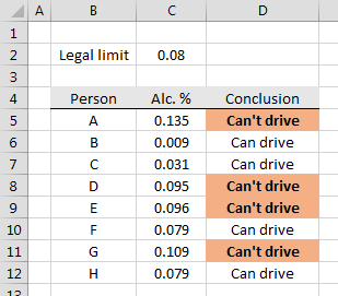
It is very easy to make cells "pop out" if they need attention. Let's take a simple example where you need to determine whether a alcohol influenced person is below the legal limit or not.

 

 

A simple IF-statement can make the text "Can't drive" or "Can drive" in the Conclusion column. However, it would be better if we could make the cells containing "Can't drive" more visible.

 

Select the cells you want to format and go to the 'Home' tab and on the 'Styles' pane you will find 'Conditional Formatting'. Select 'New Rule...'.

 

 

Then you select 'Format only cell that contain'. In this case I chose 'Specific Text' and 'containing'. You can adjust this to suit your case. Click format to change the appearance of the cell.

 



 

 

This is the result.

How to use auto fill in Excel 2013 without formatting

This is probably the most annoying default setting in Excel 2013 (and also all other versions) since it's rarely the case that I want to use the default setting of this one. A table often have columns which is just a function of other column. You edit the first line and want to auto fill the rest to the bottom of the table. But if the first line has a border, then this border is copied along making the table ugly.

 

 

Say I want column 4 to auto fill from 1, 2, 3, 4 and so on to the end. Drag and click and the following is your result.

 

 

It copies the top border line of my first cell. It assumes that it should repeat this pattern every third cell, which clearly isn't my intention. But if you click the little box which appears afterwards you can select the option 'Fill Without Formatting'.

 

 

And the result is the way you want it. It's cumbersome, but it works.

How to change the selection direction in Excel 2013 when pressing Enter

By default Excel moves the active marker down when you hit Enter. If you for some reason want to change this you can easily do that.

This can be useful if your data is structured horizontally (or any other direction).

Go to 'File' and select 'Options'. Go to the 'Advanced' tab and under 'Editing options' you can find a checkbox for 'After pressing Enter, move selection' and a drop down menu where you can select your desired direction.

If the checkbox is unchecked it will stay in the same cell when you press Enter. Select between:

• Down
• Right
• Up
• Left

How to turn off automatic calculation in Excel 2013

There are many reasons why you would want to turn of automatic calculation in Excel. One reason I often meet is when my spreadsheet uses randomly generated numbers or if I have huge spreadsheets which take some times every time it refreshes its calculations.

To turn off go to 'File', then 'Options'. Select the 'Formulas' tab and under 'Calculation options' you will find three options:

• Automatic
• Automatic except for data tables
• Manual

Under manual you can select 'Recalculate workbook before saving'. Use this if you want Excel to refresh all values before saving your workbook.

When 'Manual' is selected you can refresh either with the 'F9' key or by clicking 'Calculate Now' under the 'Formulas' tab.